pandas Guide#
This is an elegant-design introduction to pandas, geared mainly for new users. You can see more complex recipes at pandas. Note that this introduction refers to the official documentation, so pandas has copyright to part of the content. The author enhances by adding more detailed examples and explanations for easier comprehension.
Customarily, we import as follows:
In [1]: import numpy as np

In [2]: import pandas as pd
Object creation#
Creating a Series by passing a list of values, letting pandas create a default integer index:
In [3]: s = pd.Series([1, 3, 5, np.nan, 6, 8]); s
Out[3]:
0    1.0
1    3.0
2    5.0
3    NaN
4    6.0
5    8.0
dtype: float64
Creating a DataFrame by passing a Numpy array, with a datetime index and labeled columns:
In [4]: dates = pd.date_range("20210801", periods=6)

In [5]: dates
Out[5]:
DatetimeIndex(['2021-08-01', '2021-08-02', '2021-08-03', '2021-08-04',
               '2021-08-05', '2021-08-06'],
              dtype='datetime64[us]', freq='D')

In [6]: df = pd.DataFrame(np.random.randn(6, 4), index=dates, columns=list("ABCD"))

In [7]: df
Out[7]:
                   A         B         C         D
2021-08-01  0.496714 -0.138264  0.647689  1.523030
2021-08-02 -0.234153 -0.234137  1.579213  0.767435
2021-08-03 -0.469474  0.542560 -0.463418 -0.465730
2021-08-04  0.241962 -1.913280 -1.724918 -0.562288
2021-08-05 -1.012831  0.314247 -0.908024 -1.412304
2021-08-06  1.465649 -0.225776  0.067528 -1.424748
Creating a DataFrame by passing a dict of objects that can be converted to series-like:
In [8]: df2 = pd.DataFrame(
   ...:     {
   ...:         "A": 4.0,
   ...:         "B": pd.Timestamp("20210801"),
   ...:         "C": pd.Series(1, index=list(range(4)), dtype="float64"),
   ...:         "D": np.array([3] * 4, dtype="int64"),
   ...:         "E": pd.Categorical(["test", "train", "test", "train"]),
   ...:         "F": "cat",
   ...:     }
   ...: )
   ...:

In [9]: df2
Out[9]:
     A          B    C  D      E    F
0  4.0 2021-08-01  1.0  3   test  cat
1  4.0 2021-08-01  1.0  3  train  cat
2  4.0 2021-08-01  1.0  3   test  cat
3  4.0 2021-08-01  1.0  3  train  cat
The columns of the resulting DataFrame have different dtypes:
In [10]: df2.dtypes
Out[10]:
A           float64
B    datetime64[us]
C           float64
D             int64
E          category
F               str
dtype: object
or the data type for a specific column:
In [11]: df2.A.dtype
Out[11]: dtype('float64')
If you’re using IPython, tab completion for public attributes is automatically enabled. Here’s a subset of the attributes that will be completed:
In [12]: df2.<TAB>  # noqa: E225, E999
df2.A                  df2.bool
df2.abs                df2.boxplot
df2.add                df2.C
df2.add_prefix         df2.clip
df2.add_suffix         df2.columns
df2.align              df2.copy
df2.all                df2.count
df2.any                df2.combine
df2.append             df2.D
df2.apply              df2.describe
df2.applymap           df2.diff
df2.B                  df2.duplicated
Viewing data#
Here is how to view the top and bottom rows of the frame:
In [13]: df.head()
Out[13]:
                   A         B         C         D
2021-08-01  0.496714 -0.138264  0.647689  1.523030
2021-08-02 -0.234153 -0.234137  1.579213  0.767435
2021-08-03 -0.469474  0.542560 -0.463418 -0.465730
2021-08-04  0.241962 -1.913280 -1.724918 -0.562288
2021-08-05 -1.012831  0.314247 -0.908024 -1.412304

In [14]: df.tail(3)
Out[14]:
                   A         B         C         D
2021-08-04  0.241962 -1.913280 -1.724918 -0.562288
2021-08-05 -1.012831  0.314247 -0.908024 -1.412304
2021-08-06  1.465649 -0.225776  0.067528 -1.424748
Display the index, columns:
In [15]: df.index
Out[15]:
DatetimeIndex(['2021-08-01', '2021-08-02', '2021-08-03', '2021-08-04',
               '2021-08-05', '2021-08-06'],
              dtype='datetime64[us]', freq='D')

In [16]: df.columns
Out[16]: Index(['A', 'B', 'C', 'D'], dtype='str')
Display the shape, dimension:
In [17]: df.shape
Out[17]: (6, 4)

In [18]: df.ndim
Out[18]: 2
Note
DataFrame.to_numpy gives a Numpy representation of the underlying data.Note that this can be an expensive operation when your DataFrame has columns with different data types, which comes down to a fundamental difference between pandas and Numpy: Numpy arrays have one dtype for the entire array, while pandas DataFrames have one dtype per column. When you call DataFrame.to_numpy, pandas will find the Numpy dtype that can hold all of the dtypes in the DataFrame. This may end up being object, which requires casting every value to a Python object.
For df, our DataFrame of all floating-point values, DataFrame.to_numpy is fast and doesn’t require copying data.
In [19]: df.to_numpy()
Out[19]:
array([[ 0.4967, -0.1383,  0.6477,  1.523 ],
       [-0.2342, -0.2341,  1.5792,  0.7674],
       [-0.4695,  0.5426, -0.4634, -0.4657],
       [ 0.242 , -1.9133, -1.7249, -0.5623],
       [-1.0128,  0.3142, -0.908 , -1.4123],
       [ 1.4656, -0.2258,  0.0675, -1.4247]])
For df2, the DataFrame with multiple dtypes, DataFrame.to_numpy is relatively expensive.
In [20]: df2.to_numpy()
Out[20]:
array([[4.0, Timestamp('2021-08-01 00:00:00'), 1.0, 3, 'test', 'cat'],
       [4.0, Timestamp('2021-08-01 00:00:00'), 1.0, 3, 'train', 'cat'],
       [4.0, Timestamp('2021-08-01 00:00:00'), 1.0, 3, 'test', 'cat'],
       [4.0, Timestamp('2021-08-01 00:00:00'), 1.0, 3, 'train', 'cat']],
      dtype=object)
Note
DataFrame.to_numpy does not include the index or column labels in the output.
DataFrame.describe shows a quick statistic summary of your data:
In [21]: df.describe()
Out[21]:
              A         B         C         D
count  6.000000  6.000000  6.000000  6.000000
mean   0.081311 -0.275775 -0.133655 -0.262434
std    0.861950  0.862828  1.168366  1.187681
min   -1.012831 -1.913280 -1.724918 -1.424748
25%   -0.410644 -0.232047 -0.796872 -1.199800
50%    0.003904 -0.182020 -0.197945 -0.514009
75%    0.433026  0.201119  0.502648  0.459144
max    1.465649  0.542560  1.579213  1.523030
DateFrame.info show information about dataset
In [22]: df.info()
<class 'pandas.DataFrame'>
DatetimeIndex: 6 entries, 2021-08-01 to 2021-08-06
Freq: D
Data columns (total 4 columns):
 #   Column  Non-Null Count  Dtype
---  ------  --------------  -----
 0   A       6 non-null      float64
 1   B       6 non-null      float64
 2   C       6 non-null      float64
 3   D       6 non-null      float64
dtypes: float64(4)
memory usage: 240.0 bytes
Locate and aggregate NaN values column-wise:
In [23]: df.isnull().sum().sort_values(ascending=False)
Out[23]:
A    0
B    0
C    0
D    0
dtype: int64
Find the total number of NaN values
In [24]: df.isna().sum().sum() # identical to isnull() here
Out[24]: np.int64(0)
Transposing your data:
In [25]: df.T
Out[25]:
   2021-08-01  2021-08-02  2021-08-03  2021-08-04  2021-08-05  2021-08-06
A    0.496714   -0.234153   -0.469474    0.241962   -1.012831    1.465649
B   -0.138264   -0.234137    0.542560   -1.913280    0.314247   -0.225776
C    0.647689    1.579213   -0.463418   -1.724918   -0.908024    0.067528
D    1.523030    0.767435   -0.465730   -0.562288   -1.412304   -1.424748
Sorting by an axis:
In [26]: df.sort_index(axis=1, ascending=False)
Out[26]:
                   D         C         B         A
2021-08-01  1.523030  0.647689 -0.138264  0.496714
2021-08-02  0.767435  1.579213 -0.234137 -0.234153
2021-08-03 -0.465730 -0.463418  0.542560 -0.469474
2021-08-04 -0.562288 -1.724918 -1.913280  0.241962
2021-08-05 -1.412304 -0.908024  0.314247 -1.012831
2021-08-06 -1.424748  0.067528 -0.225776  1.465649
Sorting by values:
In [27]: df.sort_values(by="B")
Out[27]:
                   A         B         C         D
2021-08-04  0.241962 -1.913280 -1.724918 -0.562288
2021-08-02 -0.234153 -0.234137  1.579213  0.767435
2021-08-06  1.465649 -0.225776  0.067528 -1.424748
2021-08-01  0.496714 -0.138264  0.647689  1.523030
2021-08-05 -1.012831  0.314247 -0.908024 -1.412304
2021-08-03 -0.469474  0.542560 -0.463418 -0.465730
Selection#
Note
While standard Python / Numpy expressions for selecting and setting are intuitive and come in handy for interactive work, for production code, we recommend the optimized pandas data access methods, .at, .iat, .loc and .iloc.
Getting#
Selecting a single column, which yields a Series, equivalent to df.A:
In [28]: df["A"]
Out[28]:
2021-08-01    0.496714
2021-08-02   -0.234153
2021-08-03   -0.469474
2021-08-04    0.241962
2021-08-05   -1.012831
2021-08-06    1.465649
Freq: D, Name: A, dtype: float64
Selecting via [], which slices the rows.
In [29]: df[0:3]
Out[29]:
                   A         B         C         D
2021-08-01  0.496714 -0.138264  0.647689  1.523030
2021-08-02 -0.234153 -0.234137  1.579213  0.767435
2021-08-03 -0.469474  0.542560 -0.463418 -0.465730

In [30]: df["20210802":"20210804"]
Out[30]:
                   A         B         C         D
2021-08-02 -0.234153 -0.234137  1.579213  0.767435
2021-08-03 -0.469474  0.542560 -0.463418 -0.465730
2021-08-04  0.241962 -1.913280 -1.724918 -0.562288
Selection by label#
For getting a cross section using a label:
In [31]: df.loc[dates[0]]
Out[31]:
A    0.496714
B   -0.138264
C    0.647689
D    1.523030
Name: 2021-08-01 00:00:00, dtype: float64
Selecting on a multi-axis by label:
In [32]: df.loc[:, ["A", "B"]]
Out[32]:
                   A         B
2021-08-01  0.496714 -0.138264
2021-08-02 -0.234153 -0.234137
2021-08-03 -0.469474  0.542560
2021-08-04  0.241962 -1.913280
2021-08-05 -1.012831  0.314247
2021-08-06  1.465649 -0.225776
Showing label slicing, both endpoints are included:
In [33]: df.loc["20210802":"20210804", ["A", "B"]]
Out[33]:
                   A         B
2021-08-02 -0.234153 -0.234137
2021-08-03 -0.469474  0.542560
2021-08-04  0.241962 -1.913280
Reduction in the dimensions of the returned object:
In [34]: df.loc["20210802", ["A", "B"]]
Out[34]:
A   -0.234153
B   -0.234137
Name: 2021-08-02 00:00:00, dtype: float64
For getting a scalar value:
In [35]: df.loc[dates[0], "A"]
Out[35]: np.float64(0.4967141530112327)
For getting fast access to a scalar (equivalent to the prior method):
In [36]: df.at[dates[0], "A"]
Out[36]: np.float64(0.4967141530112327)
Selection by position#
Select via the position of the passed integers:
In [37]: df.iloc[3]
Out[37]:
A    0.241962
B   -1.913280
C   -1.724918
D   -0.562288
Name: 2021-08-04 00:00:00, dtype: float64
By integer slices, acting similar to Numpy/Python:
In [38]: df.iloc[3:5, 0:2]
Out[38]:
                   A         B
2021-08-04  0.241962 -1.913280
2021-08-05 -1.012831  0.314247
By lists of integer position locations, similar to the Numpy/Python style:
In [39]: df.iloc[[1, 2, 4], [0, 2]]
Out[39]:
                   A         C
2021-08-02 -0.234153  1.579213
2021-08-03 -0.469474 -0.463418
2021-08-05 -1.012831 -0.908024
For slicing rows explicitly:
In [40]: df.iloc[1:3, :]
Out[40]:
                   A         B         C         D
2021-08-02 -0.234153 -0.234137  1.579213  0.767435
2021-08-03 -0.469474  0.542560 -0.463418 -0.465730
For slicing columns explicitly:
In [41]: df.iloc[:, 1:3]
Out[41]:
                   B         C
2021-08-01 -0.138264  0.647689
2021-08-02 -0.234137  1.579213
2021-08-03  0.542560 -0.463418
2021-08-04 -1.913280 -1.724918
2021-08-05  0.314247 -0.908024
2021-08-06 -0.225776  0.067528
For getting a value explicitly:
In [42]: df.iloc[1, 1]
Out[42]: np.float64(-0.23413695694918055)
For getting fast access to a scalar (equivalent to the prior method):
In [43]: df.iat[1, 1]
Out[43]: np.float64(-0.23413695694918055)
Selection by dtype#
In [44]: titanic = pd.DataFrame(
   ....:     {
   ....:         "age": [22, 38, 26, 35],
   ....:         "fare": [7.25, 71.28, 7.92, 53.10],
   ....:         "name": ["Allen", "Cumings", "Heikkinen", "Futrelle"],
   ....:         "survived": [0, 1, 1, 1],
   ....:         "embarked": ["S", "C", "S", "S"],
   ....:     }
   ....: )
   ....:

In [45]: titanic.head()
Out[45]:
   age   fare       name  survived embarked
0   22   7.25      Allen         0        S
1   38  71.28    Cumings         1        C
2   26   7.92  Heikkinen         1        S
3   35  53.10   Futrelle         1        S

In [46]: titanic.select_dtypes(include=['datetime', 'number']).head()
Out[46]:
   age   fare  survived
0   22   7.25         0
1   38  71.28         1
2   26   7.92         1
3   35  53.10         1

In [47]: titanic.select_dtypes(exclude=['object', 'double']).head()
Out[47]:
   age  survived
0   22         0
1   38         1
2   26         1
3   35         1
Boolean indexing#
Using a single column’s values to select data.
In [48]: df[df["A"] > 0]
Out[48]:
                   A         B         C         D
2021-08-01  0.496714 -0.138264  0.647689  1.523030
2021-08-04  0.241962 -1.913280 -1.724918 -0.562288
2021-08-06  1.465649 -0.225776  0.067528 -1.424748
Selecting values from a DataFrame where a boolean condition is met.
In [49]: df[df > 0]
Out[49]:
                   A         B         C         D
2021-08-01  0.496714       NaN  0.647689  1.523030
2021-08-02       NaN       NaN  1.579213  0.767435
2021-08-03       NaN  0.542560       NaN       NaN
2021-08-04  0.241962       NaN       NaN       NaN
2021-08-05       NaN  0.314247       NaN       NaN
2021-08-06  1.465649       NaN  0.067528       NaN
Using the Series.isin method for filtering:
In [50]: df2[df2["E"].isin(["test"])]
Out[50]:
     A          B    C  D     E    F
0  4.0 2021-08-01  1.0  3  test  cat
2  4.0 2021-08-01  1.0  3  test  cat
Setting#
Setting a new column automatically aligns the data by the indexes.
In [51]: s1 = pd.Series(np.arange(6)+1, index=pd.date_range("20210801", periods=6))

In [52]: s1
Out[52]:
2021-08-01    1
2021-08-02    2
2021-08-03    3
2021-08-04    4
2021-08-05    5
2021-08-06    6
Freq: D, dtype: int64

In [53]: df["F"] = s1
Setting values by label:
In [54]: df.at[dates[0], "A"] = 0
Setting values by position:
In [55]: df.iat[0, 1] = 0
Setting by assigning with a Numpy array:
In [56]: df["D"] = np.array([6] * len(df))
The result of the prior setting operations.
In [57]: df
Out[57]:
                   A         B         C  D  F
2021-08-01  0.000000  0.000000  0.647689  6  1
2021-08-02 -0.234153 -0.234137  1.579213  6  2
2021-08-03 -0.469474  0.542560 -0.463418  6  3
2021-08-04  0.241962 -1.913280 -1.724918  6  4
2021-08-05 -1.012831  0.314247 -0.908024  6  5
2021-08-06  1.465649 -0.225776  0.067528  6  6
A where operation with setting.
In [58]: df2 = df.copy()

In [59]: df2[df2 > 0] = -df2

In [60]: df2
Out[60]:
                   A         B         C  D  F
2021-08-01  0.000000  0.000000 -0.647689 -6 -1
2021-08-02 -0.234153 -0.234137 -1.579213 -6 -2
2021-08-03 -0.469474 -0.542560 -0.463418 -6 -3
2021-08-04 -0.241962 -1.913280 -1.724918 -6 -4
2021-08-05 -1.012831 -0.314247 -0.908024 -6 -5
2021-08-06 -1.465649 -0.225776 -0.067528 -6 -6
Missing data#
pandas primarily uses the value np.nan to represent missing data. It is by default not included in computations.
Reindexing allows you to change/add/delete the index on a specified axis. This returns a copy of the data.
In [61]: df1 = df.reindex(index=dates[0:4], columns=list(df.columns) + ["E"])

In [62]: df1
Out[62]:
                   A         B         C  D  F   E
2021-08-01  0.000000  0.000000  0.647689  6  1 NaN
2021-08-02 -0.234153 -0.234137  1.579213  6  2 NaN
2021-08-03 -0.469474  0.542560 -0.463418  6  3 NaN
2021-08-04  0.241962 -1.913280 -1.724918  6  4 NaN

In [63]: df1.loc[dates[0] : dates[1], "E"] = 1

In [64]: df1
Out[64]:
                   A         B         C  D  F    E
2021-08-01  0.000000  0.000000  0.647689  6  1  1.0
2021-08-02 -0.234153 -0.234137  1.579213  6  2  1.0
2021-08-03 -0.469474  0.542560 -0.463418  6  3  NaN
2021-08-04  0.241962 -1.913280 -1.724918  6  4  NaN
Drop any rows that have missing data.
In [65]: df1.dropna(how="any")
Out[65]:
                   A         B         C  D  F    E
2021-08-01  0.000000  0.000000  0.647689  6  1  1.0
2021-08-02 -0.234153 -0.234137  1.579213  6  2  1.0
Drop any columns that exceed certain threshold。
In [66]: df1.dropna(thresh=len(df)*0.9, axis=1)
Out[66]:
Empty DataFrame
Columns: []
Index: [2021-08-01 00:00:00, 2021-08-02 00:00:00, 2021-08-03 00:00:00, 2021-08-04 00:00:00]
Get the boolean mask where values are nan.
In [67]: pd.isna(df1)
Out[67]:
                A      B      C      D      F      E
2021-08-01  False  False  False  False  False  False
2021-08-02  False  False  False  False  False  False
2021-08-03  False  False  False  False  False   True
2021-08-04  False  False  False  False  False   True
Replace NaN in a column with a value.
In [68]: df1["E"] = df1.E.replace(np.nan, 6.0)

In [69]: df1
Out[69]:
                   A         B         C  D  F    E
2021-08-01  0.000000  0.000000  0.647689  6  1  1.0
2021-08-02 -0.234153 -0.234137  1.579213  6  2  1.0
2021-08-03 -0.469474  0.542560 -0.463418  6  3  6.0
2021-08-04  0.241962 -1.913280 -1.724918  6  4  6.0
Filling missing data with closest previous valid value with preceding direction
In [70]: df1.ffill(axis=0)  # previous row -> current row, fill from above
Out[70]:
                   A         B         C  D  F    E
2021-08-01  0.000000  0.000000  0.647689  6  1  1.0
2021-08-02 -0.234153 -0.234137  1.579213  6  2  1.0
2021-08-03 -0.469474  0.542560 -0.463418  6  3  6.0
2021-08-04  0.241962 -1.913280 -1.724918  6  4  6.0

In [71]: df1.ffill(axis=1)  # previous col -> current col, fill from left
Out[71]:
                   A         B         C    D    F    E
2021-08-01  0.000000  0.000000  0.647689  6.0  1.0  1.0
2021-08-02 -0.234153 -0.234137  1.579213  6.0  2.0  1.0
2021-08-03 -0.469474  0.542560 -0.463418  6.0  3.0  6.0
2021-08-04  0.241962 -1.913280 -1.724918  6.0  4.0  6.0

In [72]: df1.bfill(axis=0)  # next row -> current row, fill from below
Out[72]:
                   A         B         C  D  F    E
2021-08-01  0.000000  0.000000  0.647689  6  1  1.0
2021-08-02 -0.234153 -0.234137  1.579213  6  2  1.0
2021-08-03 -0.469474  0.542560 -0.463418  6  3  6.0
2021-08-04  0.241962 -1.913280 -1.724918  6  4  6.0

In [73]: df1.bfill(axis=1)  # next col -> current col, fill from right
Out[73]:
                   A         B         C    D    F    E
2021-08-01  0.000000  0.000000  0.647689  6.0  1.0  1.0
2021-08-02 -0.234153 -0.234137  1.579213  6.0  2.0  1.0
2021-08-03 -0.469474  0.542560 -0.463418  6.0  3.0  6.0
2021-08-04  0.241962 -1.913280 -1.724918  6.0  4.0  6.0
Drop duplicate values in a column.
In [74]: df1.drop_duplicates(subset="E", keep="last")
Out[74]:
                   A         B         C  D  F    E
2021-08-02 -0.234153 -0.234137  1.579213  6  2  1.0
2021-08-04  0.241962 -1.913280 -1.724918  6  4  6.0
Drop rows which contains a value.
In [75]: df1[((df1 != 2) & (df1 != 3)).all(axis=1)]
Out[75]:
                   A        B         C  D  F    E
2021-08-01  0.000000  0.00000  0.647689  6  1  1.0
2021-08-04  0.241962 -1.91328 -1.724918  6  4  6.0
Change certain column names.
In [76]: df1.rename(columns={"F":"Rank", "E":"Variance"})
Out[76]:
                   A         B         C  D  Rank  Variance
2021-08-01  0.000000  0.000000  0.647689  6     1       1.0
2021-08-02 -0.234153 -0.234137  1.579213  6     2       1.0
2021-08-03 -0.469474  0.542560 -0.463418  6     3       6.0
2021-08-04  0.241962 -1.913280 -1.724918  6     4       6.0
Operations#
Stats#
Operations in general exclude missing data.
Performing a descriptive statistic:
In [77]: df.mean()
Out[77]:
A   -0.001475
B   -0.252731
C   -0.133655
D    6.000000
F    3.500000
dtype: float64
Same operation on the other axis:
In [78]: df.mean(axis=1)
Out[78]:
2021-08-01    1.529538
2021-08-02    1.822184
2021-08-03    1.721934
2021-08-04    1.320753
2021-08-05    1.878678
2021-08-06    2.661480
Freq: D, dtype: float64
Operating with objects that have different dimensionality and need alignment. In addition, pandas automatically broadcasts along the specified dimension.
In [79]: s = pd.Series([1, 3, 5, np.nan, 6, 8], index=dates).shift(2)

In [80]: s
Out[80]:
2021-08-01    NaN
2021-08-02    NaN
2021-08-03    1.0
2021-08-04    3.0
2021-08-05    5.0
2021-08-06    NaN
Freq: D, dtype: float64

In [81]: df.sub(s, axis="index")
Out[81]:
                   A         B         C    D    F
2021-08-01       NaN       NaN       NaN  NaN  NaN
2021-08-02       NaN       NaN       NaN  NaN  NaN
2021-08-03 -1.469474 -0.457440 -1.463418  5.0  2.0
2021-08-04 -2.758038 -4.913280 -4.724918  3.0  1.0
2021-08-05 -6.012831 -4.685753 -5.908024  1.0  0.0
2021-08-06       NaN       NaN       NaN  NaN  NaN
Apply#
Applying functions to the data:
In [82]: df.apply(np.cumsum)
Out[82]:
                   A         B         C   D   F
2021-08-01  0.000000  0.000000  0.647689   6   1
2021-08-02 -0.234153 -0.234137  2.226901  12   3
2021-08-03 -0.703628  0.308423  1.763484  18   6
2021-08-04 -0.461665 -1.604857  0.038566  24  10
2021-08-05 -1.474497 -1.290610 -0.869458  30  15
2021-08-06 -0.008848 -1.516386 -0.801930  36  21

In [83]: df.apply(lambda x: x.max() - x.min())
Out[83]:
A    2.478480
B    2.455840
C    3.304131
D    0.000000
F    5.000000
dtype: float64
String Methods#
Series is equipped with a set of string processing methods in the str attribute that make it easy to operate on each element of the array, as in the code snippet below. Note that pattern-matching in str generally uses regular expressions by default (and in some cases always uses them).
In [84]: s = pd.Series(["A", "B", "C", np.nan, "CABA", "dog", "cat"])

In [85]: s.str.lower()
Out[85]:
0       a
1       b
2       c
3     NaN
4    caba
5     dog
6     cat
dtype: str
More string methods are provided like str.title, str.capitalize, str.upper.
Data types#
Several methods to convert data types are available:
In [86]: df = pd.DataFrame({
   ....:    'product': ['A', 'B', 'C', 'D'],
   ....:    'price': ['10', '20', '30', '40'],
   ....:    'sales': ['20', '-', '60', '-']
   ....: })
   ....:

In [87]: df
Out[87]:
  product price sales
0       A    10    20
1       B    20     -
2       C    30    60
3       D    40     -

In [88]: df = df.astype({'price': 'int'})
But when we use astype to convert sales to integer, ValueError will occur because of invalid literal ‘-’. Fortunately, to_numeric solves the issue with parameter errors:
In [89]: df['sales'] = pd.to_numeric(df['sales'], errors='coerce')

In [90]: df.dtypes
Out[90]:
product        str
price        int64
sales      float64
dtype: object
Merge#
Join#
We illustrate a more detailed example in a background of business. Suppose we have three dataframes:
In [91]: df1 = pd.DataFrame({
   ....:    "id": np.arange(1, 4),
   ....:    "price": [99, 105, 50]
   ....: })
   ....:

In [92]: df1
Out[92]:
   id  price
0   1     99
1   2    105
2   3     50

In [93]: df2 = pd.DataFrame({
   ....:    "id": np.arange(3, 5),
   ....:    "count": [12, 15]
   ....: })
   ....:

In [94]: df2
Out[94]:
   id  count
0   3     12
1   4     15

In [95]: df3 = pd.DataFrame({
   ....:    "id": np.arange(1, 7),
   ....:    "price": [99, 105, 50, 60, 30, 40],
   ....:    "count": [10, 20, 12, 15, 100, 50],
   ....:    "date": pd.date_range("20210801", periods=6)
   ....: })
   ....:

In [96]: df3
Out[96]:
   id  price  count       date
0   1     99     10 2021-08-01
1   2    105     20 2021-08-02
2   3     50     12 2021-08-03
3   4     60     15 2021-08-04
4   5     30    100 2021-08-05
5   6     40     50 2021-08-06
SQL style merges :
In [97]: pd.merge(df1, df2, on="id", how="left")
Out[97]:
   id  price  count
0   1     99    NaN
1   2    105    NaN
2   3     50   12.0

In [98]: pd.merge(df1, df2, on="id", how="right")
Out[98]:
   id  price  count
0   3   50.0     12
1   4    NaN     15

In [99]: pd.merge(df1, df2, on="id", how="outer")
Out[99]:
   id  price  count
0   1   99.0    NaN
1   2  105.0    NaN
2   3   50.0   12.0
3   4    NaN   15.0

In [100]: pd.merge(df1, df2, on="id", how="inner")
Out[100]:
   id  price  count
0   3     50     12

In [101]: df1.merge(df2, on="id", how="inner") # alternative syntax
Out[101]:
   id  price  count
0   3     50     12
If we are to merge two dataframes with identical column names, directly using DataFrame.join will produce an ValueError said columns overlap but no suffix specified. One approach is to specify suffix for both dataframes with respect to columns that cause the conflict:
In [102]: df1.join(df2, lsuffix="_df1", rsuffix="_df2")
Out[102]:
   id_df1  price  id_df2  count
0       1     99     3.0   12.0
1       2    105     4.0   15.0
2       3     50     NaN    NaN
Another approach is to set ahead index for both dataframes:
In [103]: df1.set_index("id").join(df2.set_index("id"))
Out[103]:
    price  count
id
1      99    NaN
2     105    NaN
3      50   12.0
Reset index while adding the old index as a new column:
In [104]: df1 = df1.set_index("id")

In [105]: df1 = df1.reset_index()

In [106]: df1
Out[106]:
   id  price
0   1     99
1   2    105
2   3     50
Concat#
pandas provides various facilities for easily combining together Series and DataFrame objects with various kinds of set logic for the indexes and relational algebra functionality in the case of join / merge-type operations.
Split into pieces and concatenate back:
In [107]: pieces = [df3[:2], df3[2:4], df3[4:]]

In [108]: pieces
Out[108]:
[   id  price  count       date
 0   1     99     10 2021-08-01
 1   2    105     20 2021-08-02,
    id  price  count       date
 2   3     50     12 2021-08-03
 3   4     60     15 2021-08-04,
    id  price  count       date
 4   5     30    100 2021-08-05
 5   6     40     50 2021-08-06]

In [109]: pd.concat(pieces)
Out[109]:
   id  price  count       date
0   1     99     10 2021-08-01
1   2    105     20 2021-08-02
2   3     50     12 2021-08-03
3   4     60     15 2021-08-04
4   5     30    100 2021-08-05
5   6     40     50 2021-08-06
Note
Adding a column to a DataFrame is relatively fast. However, adding
a row requires a copy, and may be expensive. We recommend passing a
pre-built list of records to the DataFrame constructor instead
of building a DataFrame by iteratively appending records to it.
Extend this example to consolidate former knowledge. Determine whether to supplement products:
In [110]: df3["enough"] = np.where(df3["count"] >= 50, "yes", "no")
Add level of price to expensive or cheap:
In [111]: df3.loc[(df3["price"] > 50), "level"] = "high"

In [112]: df3.loc[(df3["price"] < 51), "level"] = "low"
Use cut to categorize data by bins:
In [113]: df3['ageGroup'] = pd.cut(df3['price'], bins=[0, 40, 70, 100],
   .....:                          labels=['low', 'mid', 'high'])
   .....:
Split date into detailed unit and horizontally append to dataframe:
In [114]: df3.date = df3.date.astype(str) # avoid AttributeError

In [115]: subdate = pd.DataFrame((x.split('-') for x in df3.date), index=df3.index,
   .....:                         columns=['year','month','day'])
   .....:

In [116]: pd.concat([df3,subdate], axis=1, keys=["df3", "dates"])
Out[116]:
  df3                                               dates
   id price count        date enough level ageGroup  year month day
0   1    99    10  2021-08-01     no  high     high  2021    08  01
1   2   105    20  2021-08-02     no  high      NaN  2021    08  02
2   3    50    12  2021-08-03     no   low      mid  2021    08  03
3   4    60    15  2021-08-04     no  high      mid  2021    08  04
4   5    30   100  2021-08-05    yes   low      low  2021    08  05
5   6    40    50  2021-08-06    yes   low      low  2021    08  06
Warning
Convert data to string dtype before conducting string manipulation, or AttributeError will occur. If we do not convert df3.date ahead, an error will raise as: AttributeError: ‘Timestamp’ object has no attribute ‘split’.
Grouping#
By “group by” we are referring to a process involving one or more of the following steps:
Splitting the data into groups based on some criteria
Applying a function to each group independently
Combining the results into a data structure
In [117]: df = pd.DataFrame({
   .....:    "A": ["foo", "bar", "foo", "bar", "foo", "bar", "foo", "foo"],
   .....:    "B": ["one", "one", "two", "three", "two", "two", "one", "three"],
   .....:    "C": np.random.randn(8),
   .....:    "D": np.random.randn(8),
   .....: })
   .....:

In [118]: df
Out[118]:
     A      B         C         D
0  foo    one  0.496714 -0.469474
1  bar    one -0.138264  0.542560
2  foo    two  0.647689 -0.463418
3  bar  three  1.523030 -0.465730
4  foo    two -0.234153  0.241962
5  bar    two -0.234137 -1.913280
6  foo    one  1.579213 -1.724918
7  foo  three  0.767435 -0.562288
Grouping and then applying the pandas.core.groupby.GroupBy.sum function to the resulting groups.
In [119]: df.groupby("A").sum(numeric_only=True)
Out[119]:
            C         D
A
bar  1.150629 -1.836450
foo  3.256897 -2.978135
Grouping by multiple columns forms a hierarchical index, and again we can apply the sum function.
In [120]: df.groupby(["A", "B"]).sum(numeric_only=True)
Out[120]:
                  C         D
A   B
bar one   -0.138264  0.542560
    three  1.523030 -0.465730
    two   -0.234137 -1.913280
foo one    2.075927 -2.194392
    three  0.767435 -0.562288
    two    0.413535 -0.221455
Reshaping#
Stack#
In [121]: tuples = list(
   .....:     zip(
   .....:         *[
   .....:             ["bar", "bar", "baz", "baz", "foo", "foo", "qux", "qux"],
   .....:             ["one", "two", "one", "two", "one", "two", "one", "two"],
   .....:         ]
   .....:     )
   .....: )
   .....:

In [122]: tuples
Out[122]:
[('bar', 'one'),
 ('bar', 'two'),
 ('baz', 'one'),
 ('baz', 'two'),
 ('foo', 'one'),
 ('foo', 'two'),
 ('qux', 'one'),
 ('qux', 'two')]

In [123]: index = pd.MultiIndex.from_tuples(tuples, names=["first", "second"])

In [124]: index
Out[124]:
MultiIndex([('bar', 'one'),
            ('bar', 'two'),
            ('baz', 'one'),
            ('baz', 'two'),
            ('foo', 'one'),
            ('foo', 'two'),
            ('qux', 'one'),
            ('qux', 'two')],
           names=['first', 'second'])

In [125]: df = pd.DataFrame(np.random.randn(8, 2), index=index, columns=["A", "B"])

In [126]: df
Out[126]:
                     A         B
first second
bar   one     0.496714 -0.138264
      two     0.647689  1.523030
baz   one    -0.234153 -0.234137
      two     1.579213  0.767435
foo   one    -0.469474  0.542560
      two    -0.463418 -0.465730
qux   one     0.241962 -1.913280
      two    -1.724918 -0.562288

In [127]: df2 = df[:4]

In [128]: df2
Out[128]:
                     A         B
first second
bar   one     0.496714 -0.138264
      two     0.647689  1.523030
baz   one    -0.234153 -0.234137
      two     1.579213  0.767435
The DataFrame.stack method compresses a level in the DataFrame’s columns.
In [129]: stacked = df2.stack(future_stack=True)

In [130]: stacked
Out[130]:
first  second
bar    one     A    0.496714
               B   -0.138264
       two     A    0.647689
               B    1.523030
baz    one     A   -0.234153
               B   -0.234137
       two     A    1.579213
               B    0.767435
dtype: float64
With a stacked DataFrame or Series (having a MultiIndex as the index), the inverse operation of DataFrame.stack is DataFrame.unstack, which by default unstacks the last level:
In [131]: stacked.unstack() # unstack on the last level 2
Out[131]:
                     A         B
first second
bar   one     0.496714 -0.138264
      two     0.647689  1.523030
baz   one    -0.234153 -0.234137
      two     1.579213  0.767435

In [132]: stacked.unstack(1)
Out[132]:
second        one       two
first
bar   A  0.496714  0.647689
      B -0.138264  1.523030
baz   A -0.234153  1.579213
      B -0.234137  0.767435

In [133]: stacked.unstack(0)
Out[133]:
first          bar       baz
second
one    A  0.496714 -0.234153
       B -0.138264 -0.234137
two    A  0.647689  1.579213
       B  1.523030  0.767435
Pivot tables#
In [134]: df = pd.DataFrame(
   .....:     {
   .....:         "A": ["one", "one", "two", "three"] * 3,
   .....:         "B": ["A", "B", "C"] * 4,
   .....:         "C": ["foo", "foo", "foo", "bar", "bar", "bar"] * 2,
   .....:         "D": np.random.randn(12),
   .....:         "E": np.random.randn(12),
   .....:     }
   .....: )
   .....:

In [135]: df
Out[135]:
        A  B    C         D         E
0     one  A  foo  0.496714  0.241962
1     one  B  foo -0.138264 -1.913280
2     two  C  foo  0.647689 -1.724918
3   three  A  bar  1.523030 -0.562288
4     one  B  bar -0.234153 -1.012831
5     one  C  bar -0.234137  0.314247
6     two  A  foo  1.579213 -0.908024
7   three  B  foo  0.767435 -1.412304
8     one  C  foo -0.469474  1.465649
9     one  A  bar  0.542560 -0.225776
10    two  B  bar -0.463418  0.067528
11  three  C  bar -0.465730 -1.424748
We can produce pivot tables from this data very easily:
In [136]: pd.pivot_table(df, values="D", index=["A", "B"], columns=["C"])
Out[136]:
C             bar       foo
A     B
one   A  0.542560  0.496714
      B -0.234153 -0.138264
      C -0.234137 -0.469474
three A  1.523030       NaN
      B       NaN  0.767435
      C -0.465730       NaN
two   A       NaN  1.579213
      B -0.463418       NaN
      C       NaN  0.647689
Time series#
pandas has simple, powerful, and efficient functionality for performing resampling operations during frequency conversion (e.g., converting secondly data into 5-minutely data). This is extremely common in, but not limited to, financial applications.
In [137]: rng = pd.date_range("1/1/2012", periods=100, freq="s")

In [138]: ts = pd.Series(np.random.randint(0, 500, len(rng)), index=rng)

In [139]: ts
Out[139]:
2012-01-01 00:00:00    102
2012-01-01 00:00:01    435
2012-01-01 00:00:02    348
2012-01-01 00:00:03    270
2012-01-01 00:00:04    106
                      ...
2012-01-01 00:01:35    401
2012-01-01 00:01:36    217
2012-01-01 00:01:37     43
2012-01-01 00:01:38    161
2012-01-01 00:01:39    201
Freq: s, Length: 100, dtype: int64

In [140]: ts.resample("5min").sum()
Out[140]:
2012-01-01    25270
Freq: 5min, dtype: int64
Time zone representation:
In [141]: rng = pd.date_range("3/6/2012 00:00", periods=5, freq="D")

In [142]: ts = pd.Series(np.random.randn(len(rng)), rng)

In [143]: ts
Out[143]:
2012-03-06    0.496714
2012-03-07   -0.138264
2012-03-08    0.647689
2012-03-09    1.523030
2012-03-10   -0.234153
Freq: D, dtype: float64

In [144]: ts_utc = ts.tz_localize("UTC")

In [145]: ts_utc
Out[145]:
2012-03-06 00:00:00+00:00    0.496714
2012-03-07 00:00:00+00:00   -0.138264
2012-03-08 00:00:00+00:00    0.647689
2012-03-09 00:00:00+00:00    1.523030
2012-03-10 00:00:00+00:00   -0.234153
Freq: D, dtype: float64
Converting to another time zone:
In [146]: ts_utc.tz_convert("America/New_York")
Out[146]:
2012-03-05 19:00:00-05:00    0.496714
2012-03-06 19:00:00-05:00   -0.138264
2012-03-07 19:00:00-05:00    0.647689
2012-03-08 19:00:00-05:00    1.523030
2012-03-09 19:00:00-05:00   -0.234153
dtype: float64
Converting between time span representations:
In [147]: rng = pd.date_range("1/1/2012", periods=5, freq="ME")

In [148]: ts = pd.Series(np.random.randn(len(rng)), index=rng)

In [149]: ts
Out[149]:
2012-01-31    0.496714
2012-02-29   -0.138264
2012-03-31    0.647689
2012-04-30    1.523030
2012-05-31   -0.234153
Freq: ME, dtype: float64

In [150]: ps = ts.to_period()

In [151]: ps
Out[151]:
2012-01    0.496714
2012-02   -0.138264
2012-03    0.647689
2012-04    1.523030
2012-05   -0.234153
Freq: M, dtype: float64

In [152]: ps.to_timestamp()
Out[152]:
2012-01-01    0.496714
2012-02-01   -0.138264
2012-03-01    0.647689
2012-04-01    1.523030
2012-05-01   -0.234153
Freq: MS, dtype: float64
Converting between period and timestamp enables some convenient arithmetic functions to be used. In the following example, we convert a quarterly frequency with year ending in November to 9am of the end of the month following the quarter end:
In [153]: prng = pd.period_range("1990Q1", "2000Q4", freq="Q-NOV")

In [154]: ts = pd.Series(np.random.randn(len(prng)), prng)

In [155]: ts.index = (prng.asfreq("M", "e") + 1).asfreq("h", "s") + 9

In [156]: ts.head()
Out[156]:
1990-03-01 09:00    0.496714
1990-06-01 09:00   -0.138264
1990-09-01 09:00    0.647689
1990-12-01 09:00    1.523030
1991-03-01 09:00   -0.234153
Freq: h, dtype: float64
Categoricals#
pandas can include categorical data in a DataFrame.
In [157]: df = pd.DataFrame(
   .....:     {
   .....:         "id": [1, 2, 3, 4, 5, 6],
   .....:         "raw_grade": ["a", "b", "b", "a", "a", "e"]
   .....:      }
   .....: )
   .....:
Convert the raw grades to a categorical data type.
In [158]: df["grade"] = df["raw_grade"].astype("category")

In [159]: df["grade"]
Out[159]:
0    a
1    b
2    b
3    a
4    a
5    e
Name: grade, dtype: category
Categories (3, str): ['a', 'b', 'e']
Rename the categories to more meaningful names (assigning to Series.cat.rename_categories is in place!).
In [160]: df["grade"] = df["grade"].cat.rename_categories(["very good", "good", "very bad"])

In [161]: df["grade"]
Out[161]:
0    very good
1         good
2         good
3    very good
4    very good
5     very bad
Name: grade, dtype: category
Categories (3, str): ['very good', 'good', 'very bad']
Reorder the categories and simultaneously add the missing categories (methods under Series.cat return a new Series by default).
In [162]: df["grade"] = df["grade"].cat.set_categories(
   .....:     ["very bad", "bad", "medium", "good", "very good"]
   .....: )
   .....:

In [163]: df["grade"]
Out[163]:
0    very good
1         good
2         good
3    very good
4    very good
5     very bad
Name: grade, dtype: category
Categories (5, str): ['very bad', 'bad', 'medium', 'good', 'very good']
Sorting is per order in the categories, not lexical order.
In [164]: df.sort_values(by="grade")
Out[164]:
   id raw_grade      grade
5   6         e   very bad
1   2         b       good
2   3         b       good
0   1         a  very good
3   4         a  very good
4   5         a  very good
Grouping by a categorical column also shows empty categories.
In [165]: df.groupby("grade", observed=False).size()
Out[165]:
grade
very bad     1
bad          0
medium       0
good         2
very good    3
dtype: int64
Plotting#
We use the standard convention for referencing the matplotlib API:
In [166]: import matplotlib.pyplot as plt

In [167]: plt.close("all")
The plt.close method is used to close a figure window.
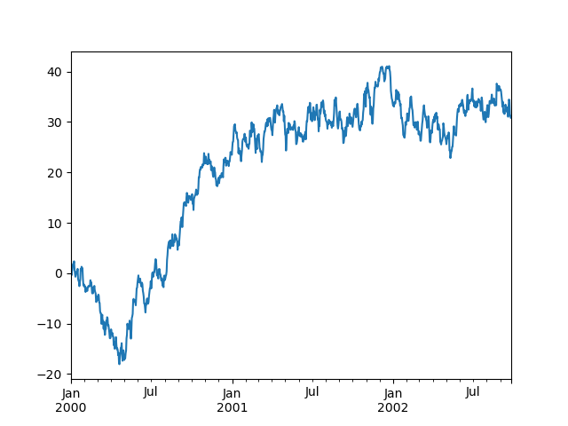
In [168]: ts = pd.Series(np.random.randn(1000), index=pd.date_range("1/1/2000", periods=1000))

In [169]: ts = ts.cumsum()

In [170]: ts.plot();
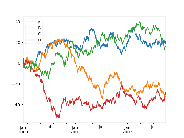
On a DataFrame, the DataFrame.plot method is a convenience to plot all of the columns with labels:
In [171]: df = pd.DataFrame(
   .....:     np.random.randn(1000, 4), index=ts.index, columns=["A", "B", "C", "D"]
   .....: )
   .....:

In [172]: df = df.cumsum()

In [173]: plt.figure();

In [174]: df.plot();

In [175]: plt.legend(loc='best');
IO Management#
CSV#
Writing to a csv file.
In [176]: df.to_csv("foo.csv")
Reading from a csv file.
In [177]: pd.read_csv("foo.csv")
Out[177]:
     Unnamed: 0          A          B         C          D
0    2000-01-01   0.496714  -0.138264  0.647689   1.523030
1    2000-01-02   0.262561  -0.372401  2.226901   2.290465
2    2000-01-03  -0.206914   0.170159  1.763484   1.824735
3    2000-01-04   0.035049  -1.743121  0.038566   1.262447
4    2000-01-05  -0.977782  -1.428874 -0.869458  -0.149856
..          ...        ...        ...       ...        ...
995  2002-09-22  32.510885  27.254392 -6.697451  30.716444
996  2002-09-23  32.753767  25.172294 -6.144302  30.168244
997  2002-09-24  34.677213  24.397679 -7.833485  29.696980
998  2002-09-25  32.701725  25.148778 -9.898568  29.725438
999  2002-09-26  30.623913  24.828480 -8.255190  30.086086

[1000 rows x 5 columns]
Excel#
Reading and writing to MS Excel.
Writing to an excel file.
In [178]: df.to_excel("foo.xlsx", sheet_name="Sheet1")
Reading from an excel file.
In [179]: pd.read_excel("foo.xlsx", "Sheet1", index_col=None, na_values=["NA"])
Out[179]:
    Unnamed: 0          A          B         C          D
0   2000-01-01   0.496714  -0.138264  0.647689   1.523030
1   2000-01-02   0.262561  -0.372401  2.226901   2.290465
2   2000-01-03  -0.206914   0.170159  1.763484   1.824735
3   2000-01-04   0.035049  -1.743121  0.038566   1.262447
4   2000-01-05  -0.977782  -1.428874 -0.869458  -0.149856
..         ...        ...        ...       ...        ...
995 2002-09-22  32.510885  27.254392 -6.697451  30.716444
996 2002-09-23  32.753767  25.172294 -6.144302  30.168244
997 2002-09-24  34.677213  24.397679 -7.833485  29.696980
998 2002-09-25  32.701725  25.148778 -9.898568  29.725438
999 2002-09-26  30.623913  24.828480 -8.255190  30.086086

[1000 rows x 5 columns]
Composition#
To compose one dataframe from multiple files, use glob library to get paths of files with random order and concatenate vertically and horizontally.
from glob import glob
files = sorted(glob("data/prefix_*.csv"))
pd.concat((pd.read_csv(file) for file in files), ignore_index=True)
pd.concat((pd.read_csv(file) for file in files), axis=1)
Miscellaneous#
Trim white spaces for object-dtype element.
for i in df:                               # traverse each column
   if pd.api.types.is_object_dtype(df[i]): # if dtype is object
      df[i] = df[i].str.strip()          # remove white space
Copy from applications like Excel and paste through pandas as a DataFrame.
pd.read_clipboard()
Data wrangling with pandas can be referenced through an official cheatsheet.