MATLAB Guide#
This is an elegant-design introduction to MATLAB, geared mainly for new users. You can see more complex recipes at MATLAB.
As for getting help, MATLAB uses help func to get brief documentation on the function func within the command window, and uses doc func to open the documentation page with external browser. Also, it uses type func for user-defined source code. When debugging, before making a fix to your code, you should always stop your debugging session first so that you can save your changes.
IO management#
Workspace IO#
save file: save current workspace to file.matload file: load variables in file.mat to the workspaceclear [var]: clear certain variable from the workspace, or clear all if not specifiedclc: clear all text from the Command Windowformat bank/short/long: set 2/4/16 digits for numeric displayedit [scriptName]: edit script or create one if not existedscriptName: run the script
Text IO#
input: gather textual input from the Command Windowdisp: display text or arrayfprintf: write data on the screenwarning: display warning message in orange, program continues to executeerror: display error message in red, program stops execution
Graphical IO#
menu: a multiple-choice dialog boxinputdlg: a dialog box with input windowuigetfile: open standard dialog box for retrieving filesmsgbox: message dialogwarndlg: warning dialogerrordlg: error dialogxlsread: import data from an Excel file
>> [num, txt] = xlsread(filename, sheetname)
>> fprintf('Cost = $%d\n', 20)
Cost = $20
>> color = menu('Choose a color', 'red', 'yellow')
>> value = inputdlg('Please enter your ID: ')
>> filename = uigetfile
>> warndlg('Divided by zero.')
Object creation#
Several methods to create MATLAB arrays are available, and we should contain homogeneous elements only for optimal efficiency. The simplest way is
>> [3 5] % row vector
>> [3;5] % column vector
>> [1, 2, 3; 4, 5, 6] % matrix
>> ndims(a) # number of dimensions
>> numel(a) # number of elements
>> size(a)  # shape of matrix
Preallocation is an option for the growth acceleration of arrays
>> rand(n)  % square matrix in U(0,1)
>> randn(n) % square matrix in N(0,1)
>> randi([upper lower], n) % square matrix in U(u,l)
>> zeros(m, n) % mxn matrix
>> ones(n) % square matrix
>> eye(n) % identity matrix
>> diag(n) % 2D diagonal matrix
In addition, we could use : and linspace to create evenly spaced vectors, and both methods’ end parameter is border-inclusive.
%  start : space : end
>>   0   :   1   :  6
%  linspace(start, end, steps)
>> linspace(  0  ,  6 ,   7  )
The results for above two methods are the same: a list of size seven counting from zero to six.
Use meshgrid to generate grid for optimal efficiency which generates two 2D matrices with identical shape
>> [x, y] = meshgrid(0:2, 0:3)
x =  0     1     2
     0     1     2
     0     1     2
     0     1     2

y =  0     0     0
     1     1     1
     2     2     2
     3     3     3
In order to make a deep copy, direct assigning the result to a new variable.
Stack matrices are easy in MATLAB, either vertical or horizontal
>> a = [0, 1, 2]
>> b = [3, 4, 5]
>> [a b] % horizontal
ans = 0 1 2 3 4 5

>> [a;b] % vertical
ans = 0   1   2
      3   4   5
To create an array of strings or a cell array, commonly used by pie chart, use curly bracket {}.
cryptoNames = {"BTC", "SNX", "YFI"}
Use height and width to get the number of rows and columns in a matrix. If we want to replace all values of the variable AAPL with 1000, use command
stockData.AAPL = 1000 * ones(height(stockData), 1)
Selection#
Important
Indexing in MATLAB starts with one.
The common method to index an array is a(start:step:stop). If we want to access the last element, use end logical value.
>> y(1:2:end, :)
ans = 0     0     0
      2     2     2
% extract the second row
>> y(2, :)
% extract the second column
>> y(1:4, 2)
>> y(1:end, 2)

>> y(1, 2) = 5 % change value
y = 0     5     0
    1     1     1
    2     2     2
    3     3     3
MATLAB uses and & , or |, not ~, equal == for logical operations with application for boolean mask, assuming identical matrix dimensions. NaN data is dangerous in that it may ruins the analytical results or graphics, which leads to unsatisfactory conclusion.
>> y(y > 1)'
ans = 2 3 5 2 3 2 3

>> y((y < 3) | (y > 4))'
ans = 0 1 2 5 1 2 0 1 2

>> y(y > 1 & y < 3)'
ans = 2 2 2

>> mask = ~(y < 3)
mask = 0   1   0
       0   0   0
       0   0   0
       1   1   1

>> y(mask)
ans = 3 5 3 3
Note
Logical operator == cannot recognize NaN since basically it is for numerical comparison. Instead, we could use isnan.
>> x = [Inf 1 2 NaN];
>> x == NaN
ans = 0 0 0 0
>> isnan(x)
ans = 0 0 0 1
Numerous is... funcitons is provided that take an array as a input and return a logical output.
Use find to generate indices that met the condition to the original ndarray.
>> criteria = find(y > 2) % indices
criteria = 4 5 8 12

>> y(criteria)
ans = 3 5 3 3
Use strcmp to check whether two strings are equal. Use isequal to test equality of two arrays, and use isequaln for the same functionality except ignoring NaN.
Use column-wise operations all or any to test whether all or any elements in a logical vector are true. Use nnz to compute the number of non-zero elements. Parse the second argument to perform operation down this dimensional argument.
>> all(y)
ans = 0 0 0
>> any(y)
ans = 1 1 1
>> any(y, 1)
>> any(y, 2)
>> any(y, 3)
>> nnz(y)
ans = 9
Control flow#
Now we illustrate the if, switch, for, and while loops
if condition
   statement 1
elseif condition
   statement 2
else
   statement 3
end
switch expression
   case value_1
      code_1
   case value_2
      code_2
   otherwise
      code_3
end
for i = 1:3
   fprintf('%i\n', i)
end
while condition
   statement 1
   statement 2
   statement 3
end
Use ctrl + c to terminate infinite loops if happens.
Missing data#
One approach to delete elements is by assigning to []
>> y(y == 0) = [] % delete and flatten
y = 1 2 3 1 2 3 1 2 3
Another approach is to extract desired elements with ismissing to locate missing data.
>> y
y = 0     0     0
    1   NaN     1
    2     2     2
    3     3   NaN
>> missingData = ismissing(y)
missingData = 0   0   0
              0   1   0
              0   0   0
              0   0   1
>> missingRows = any(missingData, 2)
missingRows = 0
              1
              0
              1
>> completeData = y(~missingRows, :)
completeData = 0     0     0
               2     2     2
Commonly, we could remove all NaN from a matrix while preserving the most data as possible and keep the matrix format by
matrix(:, all(isnan(matrix))) = [];
matrix(any(isnan(matrix), 2), :) = [];
Instead, we could interpolating missing data by using interp1, which fits one-dimensional interpolant to the data, with methods available for nearest, next, previous, pchip, spline, cubic. The output dimension is the same as x. Additional parameters like extrap could be added to perform extrapolation.
y = interp1(noNaNx, noNaNy, x, 'linear')
Mathematics#
Operations between a matrix and a scalar include +, -, *, ^, /.
Element-wise operations between matrices with broadcasting concept include +, -, .*, .^, ./ , sqrt, nthroot, power, exp, log, [trigonometry], floor, ceil, round, mod etc.
Statistical operations include max, min, sum, mean, median, std, var, cov, prctile, corr, corrcoef, .' for transpose, ' for conjugate transpose, etc. These operations are default as column-wise, we could conduct row-wise operations by func(x, 2). Note that max and min ignore NaN by default. Moreover,
*: matrix multiplication/: solve linear systems of equationsdiff: calculate differences between adjacent elements of the input[]: a placeholder to skip a parameter'omitnan': omit NaN in calculations
>> nthroot(y, 2)
ans =      0         0         0
      1.0000    1.0000    1.0000
      1.4142    1.4142    1.4142
      1.7321    1.7321    1.7321

>> [1 1; 1 1]*[2 2;2 2]
ans = 4   4
      4   4

>> [1 1; 1 1].*[2 2;2 2]
ans = 2   2
      2   2

>> mean(y)
ans = 1.5000  2.7500  1.5000

>> min(ans, [], 2, 'omitnan') % row vector
ans = 1.5000
some functions above have polymorphism for multiple outputs
>> [nrow, ncol] = size(x)
>> [xMax, idx] = max(x)
For more information about operation and special characters, check out official documentation for operation and special characters.
Statistics#
Use mdl = fitlm(X, y) function to create a MATLAB object, with more information about fitdist
mdl: A LinearModel object representing a least-squares fit of the response to the data
X: An n-by-p matrix
y: An n-by-1 matrix
An object includes both:
properties such as coefficients and residuals of the fit
methods which are functions that you can perform on the fit, such as predictions and visualizations
Use plotResiduals function to visually evaluate the quality of the fit. The default plot is histogram, we could add parameters to sprcify a graph like probability, lagged, fitted, symmetry, caseorder.
>> AAPLfit = fitlm(daysNum, AAPL);
>> plot(dates, AAPL);
>> hold on
>> plot(dates, predict(AAPLfit, daysNum))
>> plotResiduals(AAPLfit)
Use plotDiagnostics function on your fit to help assess your fit visually.
>> plotDiagnostics(FTSEfit,'cookd')
Use properties to view available properties.
>> properties(FTSEfit)

Properties for class LinearModel:

   Residuals
   Fitted
   Diagnostics
   MSE
   Robust
   RMSE
   Formula
   LogLikelihood
   DFE
   SSE
   SST
   SSR
   CoefficientCovariance
   CoefficientNames
   NumCoefficients
   NumEstimatedCoefficients
   Coefficients
   Rsquared
   ModelCriterion
   VariableInfo
   NumVariables
   VariableNames
   NumPredictors
   PredictorNames
   ResponseName
   NumObservations
   Steps
   ObservationInfo
   Variables
Use predict function to predict the reponse values given any predictor values. Note that the predictor values should be stored in a column vector.
>> y = predict(modelName, (1:300)'); % predict future 200 days
We can apply different tests for normality on the raw residuals, generally having the following form: [h, p] = distributionTest(x). We illustrate by using the jbtest function, which uses the Jarque-Bera normality test, on the raw residual data.
>> [hJB, pJB] = jbtest(res)
hJB = 1         % reject H_0
pJB = 1.000e-03 % reject H_0
Use pd = fitdist(x, distname) function creates a MATLAB probability distribution object
pd: A probability distribution objectx: A column vector of data used to calculate the fit parametersdistname: A string which identifies the probability distribution to model
Use icdf function to determine the inverse cdf value of the fit at a given value
>> tFit = fitdist(AAPLReturns, 'tLocationScale')
>> VaR99 = icdf(tFit, 0.01)
Use histogram function, you can normalize your display in many different ways using the Normalization property
>> histogram(FTSEreturns, binEdges, 'Normalization', 'pdf')
Use pdf function to determine the pdf value of the fit with a given input vector.
>> edgeBins = -0.1:0.0005:0.1
>> p = pdf(tFit, edgeBins)
>> plot(edgeBins, p, 'r')
You can actually generate random numbers from your data using your probability distribution object with random function. The simulated values that are generated are not simply sampled from the data, but generated from the fitted distribution. Use rng function with a nonnegative integer seed to start the random number generator in a specific spot.
>> rng('shuffle')
>> randomVector = random(tFit, rows, cols)
Functions#
Use function keyword to customize functions with end keyword to terminate the process. The example below illustrates an example of getting biggest and smallest N number in a vector
getTails(x, 3) % function call

function [topN, bottomN] = getTails(v, N)
sortedv = sort(v, 'descend');
topN = sortedv(1:N);
bottomN = sortedv(end : -1 : end-N+1);
end
Note
Function definitions in a script must appear at the end of the file. Functions have their own function workspace, which is independent from base workspace. So, while function is run, it cannot access variables in the base workspace and other functions’ workspaces.
By default, we can call functions in which folder the current file locates. If you want to access the files in the other folders, you can add the folders in MATLAB’s search path by ENVIRONMENT -> Set Path in the manu bar.
MATLAB has calling precedence. If two named item have the same name, an order as a set of rules is applied as
Variables
Files in the current folder
Files on MATLAB search path
We can use which command to check the item location and property in the precedence order. Suppose we have a variable named var as a VaR double,
>> which var -all
var is a variable.
.../MATLAB_R2021b/.../bigdata/var.m     % Shadowed tall method
.../MATLAB_R2021b/.../timeseries/var.m  % Shadowed timeseries method
.../MATLAB_R2021b/.../datafun/var.m     % Shadowed
Graphics#
Use plot(x, y[, "format", *args]) to create line plots of numeric data, hold on to draw multiple plots on the same canvas, and hold off to create a new axes for the next plotted line. Use plotyy(x1, y1, x2, y2) to create a chart containing two separate vertical axes. For more information about plots, check out official documentation for plots.
To create multiple figures simultaneously, we use figure and make figure number k active by figure(k). To close one or more figures, we use close to close current active window, close(k) to close window number k, and close all to close all figures windows.
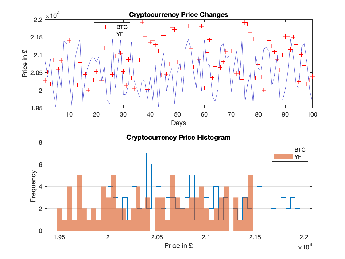
Currently, we only discuss about drawing one plot per window. If we want to create multiple axes within a single window, using subplot(m,n,k) to create an active set of axes at the kth position in an m-by-n grid . If axes already exist in this location, they are made active. The axes in the grid are numbered sequentially left-to-right, then top-to-bottom.
>> x = (1:1:100)
>> BTC = randi([20000, 22000], 100, 1)
>> YFI = randi([19500, 21500], 100, 1)
>> subplot(2, 1, 1)
>> plot(x, BTC, "r+", "LineWidth", 1)
>> hold on
>> plot(x, YFI, "Color", [0.3 0.3 0.8])
>> title("Cryptocurrency Price Changes")
>> xlabel("Days")
>> ylabel("Price in " + char(163))
>> legend("BTC", "YFI", "Location", "best")
>> xlim([1 100])
>> hold off
>> subplot(2, 1, 2)
>> histogram(BTC, 40, "DisplayStyle", "stairs")
>> hold on
>> histogram(YFI, 40, "EdgeColor", "none")
>> var = prctile(BTC, 25)
>> plot([var var], [0, 0.9])
>> title("Cryptocurrency Price Histogram")
>> xlabel("Price in " + char(163))
>> ylabel("Frequency")
>> legend("BTC", "YFI", "Location", "best")
>> grid on
>> hold off
Dates & Times#
Use datetime to represent specific dates or points in time
>> d = datetime('July 14 2021', 'InputFormat', 'MMMM dd yyyy')
d = 14-Jul-2021
>> d.Format = 'MM/dd/yyyy'
d = 07/14/2021
>> str = {'Q1 2021', 'Q2 2021'}
>> d = datetime(s, 'InputFormat', 'QQQ yyyy')
d = 01-Jan-2015   01-Apr-2015
>> t = datetime([2001, 2003, 2006], 8, 17)
t = 17-Aug-2001   17-Aug-2003   17-Aug-2006
% the month parameter may be a column vector
>> t = datetime(2007, [2;3;7;10;12], 1)
t = 01-Feb-2007
   01-Mar-2007
   01-Jul-2007
   01-Oct-2007
   01-Dec-2007
>> t1 = datetime(2015, 1, 1);
>> t2 = datetime(2015, 1, 5);
>> t = t1:t2
t = 01-Jan-2015 ... 04-Jan-2015   05-Jan-2015
>> t = linspace(t1, t2, 3)
t = 01-Jan-2015   03-Jan-2015   05-Jan-2015
Use duration represent a fixed-length time duration between dates, or from single unit duration variables years, days, hours, minutes, seconds. Note that the function years returns one year as 365.24 days (a fixed-length year).
>> t = duration(12, 0, 2, 500);
>> t.Format = 'mm:hh:ss.SSS'
t = 12:00:02.500
>> t = minutes(0:10:30)
t = 0 min   10 min   20 min   30 min
Use calendarDuration to represent a variable-length duration in calendar units, or from single unit duration variables calyears, calquarters, calmonths, calweeks, caldays
>> t = calendarDuration(1, 2, 3, 4, 5, 6)
t = 1y 2mo 3d 4h 5m 6s
>> t = calendarDuration(3:5, 1, 4:6)
t = 3y 1mo 4d   4y 1mo 5d   5y 1mo 6d
>> t1 = calyears(1) + calmonths(6)
t1 = 1y  6mo
MATLAB supports date arithmetic operations and functions between datetime and duration variables
>> t = datetime(1999, 1, 3) + duration(72, 0, 0)
t = 06-Jan-1999
>> v = (t+1:t+3)'
v = 07-Jan-1999
    08-Jan-1999
    09-Jan-1999
% number of full calendar months between t1 and t2
>> numel(t1:calmonths(1):t2) - 1
When applied to matrices, these functions work on a columnwise basis
diff: finds the differences between successive elements of a datetime or duration array, returning the output as a duration arraycaldiff: finds the differences between successive elements of a datetime array, returning the output as a calendarDuration arraybetween: finds the differences between corresponding elements of two datetime arrays, returning the output as a calendarDuration arraysdateshift: shift dates by a specific rule
>> t1 = datetime(1999, 2:4, [7, 20, 11])
t1 = 07-Feb-1999   20-Mar-1999   11-Apr-1999
>> t2 = datetime(2003, [6, 12, 3], 1)
t2 = 01-Jun-2003   01-Dec-2003   01-Mar-2003
>> x = diff(t1)
x = 984:00:00   528:00:00
>> y = caldiff(t1)
y = 1mo 13d       22d
>> z = between(t1, t2)
z = 4y 3mo 25d    4y 8mo 11d   3y 10mo 18d
>> t3 = datetime(2020, 2:4, [2, 30, 11])
t3 = 02-Feb-2020   30-Mar-2020   11-Apr-2020
>> dateshift(t3, 'start', 'month')
ans = 01-Feb-2020   01-Mar-2020   01-Apr-2020
>> dateshift(t3, 'end', 'week')
ans = 08-Feb-2020   04-Apr-2020   11-Apr-2020
By specifying output type options, we get preferable display option. For example, if we have a datetime
>> t = datetime(2021, 07, 20, 15, 00, 00)
t = 20-Jul-2021 15:00:00
the output type options could be (default listed first):
month:
monthofyear,name,shortnameweek:
weekofyear,weekofmonthday:
dayofmonth,dayofweek,dayofyear,name,shortnamesecond:
secondofminute,secondofday
Several methods to extracting date components are available:
ymd: get the year, month, and day numbers of a datetime as separate arrayshms: get the hour, minutes, and seconds of a datetime or duration as separate arrayssplit: split a calendarDuration variable into its constituent units
>> [y, m, d] = ymd(t)
>> [h, m, s] = hms(t)
>> [mth, wk] = split(t, {'months', 'weeks'})
Use axes tick labels to plot specific date format
>> plot(x, y, "DatetimeTickFormat", "MMM dd yyyy")
ALso, we could join data by dates using intersect
>> [intersection, idxA, idxB] = intersect(A, B)
with more set operators union, setxor, setdiff, etc.
Tabular Data#
If the data is organized in a tabular manner, such as in a spreadsheet, MATLAB provides the table data type. The data can be thought of as a series of observations (rows) over a set of different variables (columns). Use readtable to import data from a delimited text file
>> stockData = readtable('stockPrices.xls')
>> stockInfo = table(Ticker, Sector, Beta)
>> stockPrices = array2table(Prices, 'VariableNames', {'BA', 'BARC', 'BRBY'})
Note
We can access data in a table with dot notation or curly brackets. When using curly brackets, we can index via variable name or column number. Indexing with parentheses will return another table, not a numeric array. Three methods to access a specific column named colName below are identical
numArr = tableName.colName{:}
numArr = tableName{:, 'colName'}
numArr = tableName{:, colIdx}
To add a new variable in a table as a column, use command
>> tableName.NewVariable = variableToAdd
Use .Properties to retrieve all properties for a table, and we could modify a certain properties by assigning a new value.
>> stockData.Properties

TableProperties with properties:

            Description: ''
               UserData: []
         DimensionNames: {'Row'  'Variables'}
         VariableNames: {'ENRC'  'EXPN'  'FRES'  'GFS'  'GKN'}
   VariableDescriptions: {}
         VariableUnits: {}
      VariableContinuity: []
               RowNames: {}
      CustomProperties: No custom properties are set.
      Use addprop and rmprop to modify CustomProperties.
A function handle is a MATLAB variable that represents a function, and we use the @ symbol to create a handle to a function file and store it in a variable
>> variableName = @functionName
While one can apply a function to an array, this will lead to an error with tables. For tables, one can use a varfun function to apply a function f to all variables in a table t. The function f must take one input argument and return arrays with the same number of rows each time it is called.
>> varfun(@abs, t) % make all cells to absolute value
To work around multiple inputs, we create a wrapper function which only requires one input and others are inferred by scenarios.
function y = naninterp(y)

% create a vector of evenly spaced x-values the same length as y
x = (1:length(y))';

% create a logical vector with true at the location of non-missing values
idx = ~isnan(y);

% extract non-missing values
xClean = x(idx);
yClean = y(idx);

% use this index to extract non-missing data and interpolate the missing values
y = interp1(xClean, yClean, x, 'linear', 'extrap');

% replace missing values with interpolated values
interpData = varfun(@naninterp, data)
Use categorical to create a categorical array when text labels are intended to represent a finite set of possibilities, occupying less memory than cell arrays of strings.
Use mergecats to merge multiple cartegories into one categoty.
>> tableName.var = categorical(tableName.var)
>> c = categorical({'1', '2', '3', '4'})
c = 1 2 3 4
>> even = {'0', '2', '4', '6'}
>> c = mergecats(c, even, 'even')
c = 1 even 3 even
Use writetable to export a table to a delimited text file or Excel spreadsheet. By default, it determines the output format by file extension. No assignment operator is used.
>> writetable(tableName, 'filename.xls', 'Range', 'C5:L23')
>> writetable(tableName, 'filename.txt', 'Delimiter', '\t')
MATLAB for Finance#
Monte-Carlo and VaR#
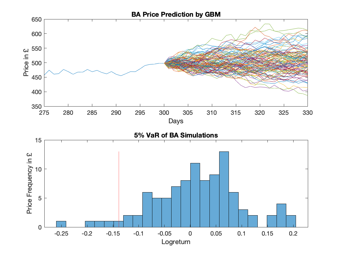
We start by illustrating predictions in stock prices using the grometric Brownian motion model (GBM). Recall the GBM equation is
Suppose to simulate 100 paths about BA with GBM using the Monte-Carlo simulation method and calculate the 5% VaR as a red line, we could write a script and generate plots
%% read data and calculate returns
>> load BA
>> stockReturns = diff(log(BA))

%% calculate the descriptive statistics
>> mu = mean(stockReturns)
>> sigma = std(stockReturns)
>> deltaT = 1
>> S0 = BA(end)

%% calculate the future prices
>> epsilon = randn(30, 100); % predict 30 days by vectorization
>> factors = exp((mu-sigma^2/2)*deltaT + sigma*epsilon*sqrt(deltaT));
>> lastPriceVector = ones(1, 100) * S0;
>> priceAndFactors = [lastPriceVector; factors]
>> paths = cumprod(priceAndFactors)

%% extract final prices, calculate returns and 5% VaR
>> finalPrices = paths(end,:);
>> possibleReturns = log(finalPrices) - log(S0);
>> var5 = prctile(possibleReturns, 5);

%% plot the paths and histogram
>> subplot(2, 1, 1)
>> plot(BA)
>> hold on
>> plot(300:330, paths)
>> xlim([275 330])
>> title("BA Price Prediction by GBM")
>> xlabel("Days")
>> ylabel("Price in " + char(163))
>> hold off
>> subplot(2, 1, 2)
>> histogram(possibleReturns, 25)
>> hold on
>> plot([var5 var5], [0 13], 'r')
>> title("5% VaR of BA Simulations")
>> xlabel("Logreturn")
>> ylabel("Price Frequency in " + char(163))
>> hold off
Formally, we could form a function to calculate the final estimated future stock price and level% VaR for maintenance purposes as
function [var, finalPrices] = calculateVaR(stock, level)

% calculate the daily log returns and the statistics
stockReturns = diff(log(stock));
mu = mean(stockReturns);
sigma = std(stockReturns);

% simulate prices for 30 days in future based on GBM
deltaT = 1;
S0 = stock(end);
epsilon = randn(30, 100);
factors = exp((mu-sigma^2/2)*deltaT + sigma*epsilon*sqrt(deltaT));
lastPriceVector = ones(1, 100) * S0;
factors2 = [lastPriceVector; factors];
paths = cumprod(factors2);

% extract final prices
finalPrices = paths(end, :);

% calculate returns
possibleReturns = log(finalPrices) - log(S0);

% calculate the VaR
var = prctile(possibleReturns, level);
Datafeed Toolbox™#
With MATLAB and Datafeed Toolbox™, you can download data from an external service provider such as Bloomberg® or FRED®.
>> c = fred; % connect to FRED server;
>> tStart = datetime(2014, 1, 1);
>> tEnd = datetime(2014, 12, 31);
>> data = fetch(c, "DJIA", tStart, tEnd);
>> DJIAData = data.Date
DJIAData = 1.0e+05 *
           7.3560       NaN
           7.3560    0.1644
             ...       ...
           7.3596    0.1782
>> DJIADates = djiaData(:, 1);
% convert the dates to the datetime format
>> DJIADates = datetime(djiaDates, "ConvertFrom", "datenum")
DJIADates = 01-Jan-2014 00:00:00   NaT
            02-Jan-2014 00:00:00   04-Jan-0045 08:24:00
                     ...                     ...
            31-Dec-2014 00:00:00   17-Oct-0048 01:40:48
>> close(c)
>> clear c
Economy Performance#
The moving average convergence/divergence (MACD) can be used as a simple indicator of the state of the economy. You can calculate the MACD by subtracting the lagging (long-term) exponential moving average from the leading (short-term) exponential moving average. Use movavg(ticker, 'exponential', n) to find the exponential moving average of n samples.
>> movAvgShort = movavg(AAPL, 'exponential', 5);
>> movAvgLong = movavg(AAPL, 'exponential', 10);
>> MACD = movAvgShort - movAvgLong;
To create a column vector named econPerformance whose elements are 1 when the economy is up, -1 when the economy is down, and 0 otherwise, we could
>> econPerformance = zeros(length(MACD), 1);
>> econPerformance(MACD >= 5) = 1;
>> econPerformance(MACD <= -5) = -1;
then extract the stock codes of all the ‘upcycle’ stocks to get the corresponding stock prices
>> upcycleIdx = strcmp(stockInfo.Classification, 'upcycle')
>> stocksToBuy = stockInfo.Code(upcycleIdx)
>> stocksToBuyPrices = stockPrices{:, stocksToBuy};
To calculate returns and remove NaNs from the output, we could
% calculate returns
stockRet = tick2ret(stockData{:,:});

% remove NaNs from stockRet
stockRet(:,all(isnan(stockRet))) = [];
stockRet(any(isnan(stockRet),2),:) = [];

% show the return values
disp('stockRet = ')
disp(stockRet)
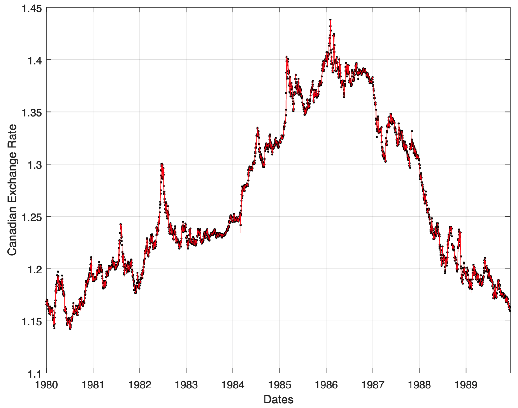
Interpolation#
Suppose we want to linearly interpolate the data from the first day to the last day in Dates and plot this data as a solid red line over the original data as black dots, we could
% import data from CanadianExchange.csv
canEx = readtable('CanadianExchange.csv');
canEx.Dates = datetime(canEx.Dates);

% plot the Canadian dollar exchange rates using black points
plot(canEx.Dates, canEx.ExchangeRate, 'k.', 'MarkerSize', 6)

% create a duration vector containing the current dates in the plot
origDays = days(canEx.Dates - canEx.Dates(1));

% create a vector of days on which to interpolate
daysI = origDays(1):origDays(end);

% interpolate the missing values
exI = interp1(origDays, canEx.ExchangeRate, daysI);

% create the interpolated date vector from the interpolated day (duration) vector
datesI = canEx.Dates(1) + daysI;

hold on
plot(datesI, exI, 'r')
xlabel('Dates')
ylabel('Canadian Exchange Rate')
grid on
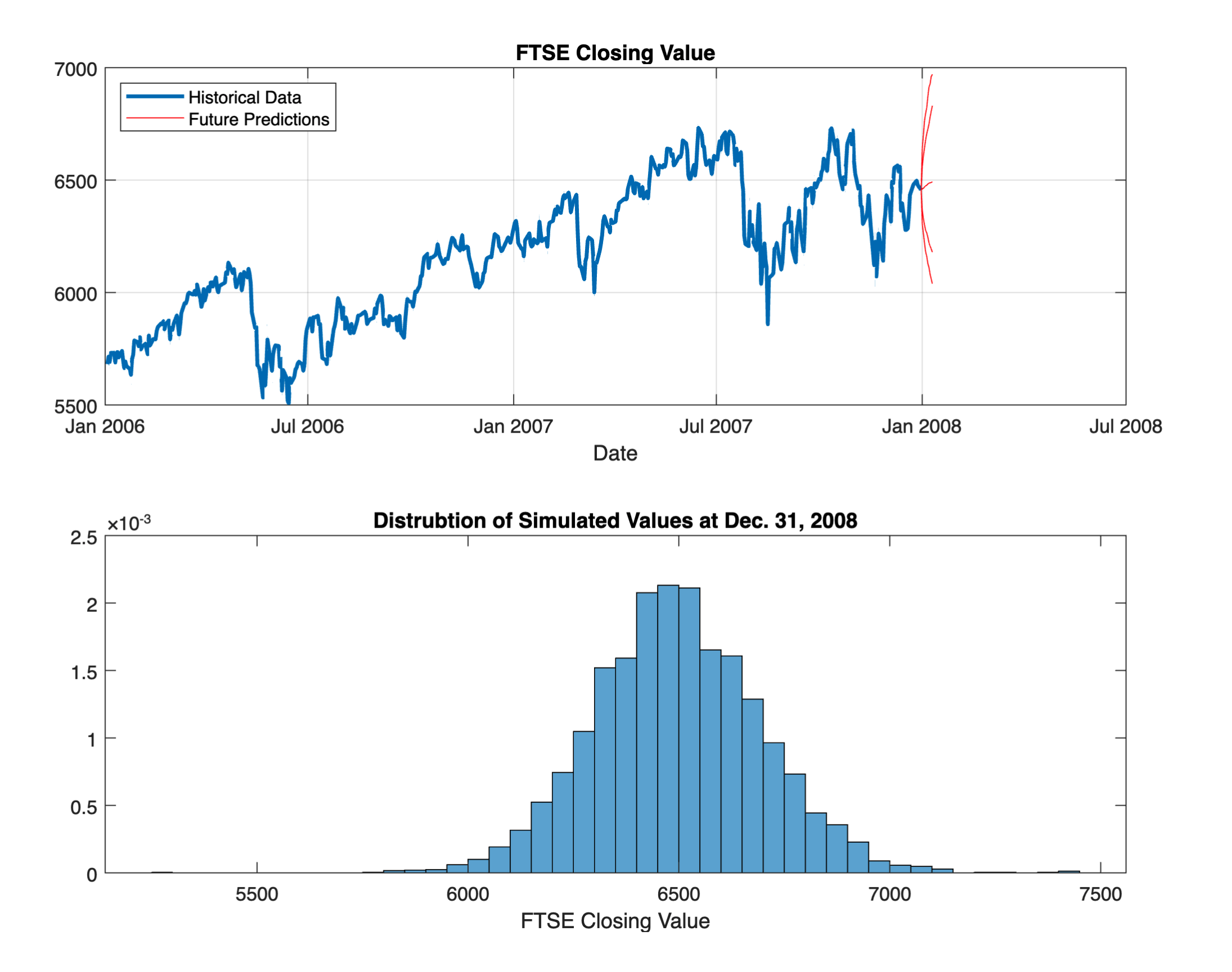
Multivariate statistics#
To create a t Location-Scale probability distribution with a fit for FTSE, we would
%% import data and compute returns
FTSEtable = readtable('FTSEavgs.csv');
FTSEtable.Dates = datetime(FTSEtable.Dates);
dys = days(datetime(FTSEtable.Dates) - datetime(FTSEtable.Dates(1)));
FTSEreturns = tick2ret(FTSEtable.FTSE, dys);

%% fit a t scale-location distribution
tFit = fitdist(FTSEreturns, 'tlocationscale');

%% Monte-Carlo Simulations for a t distribution
nSteps = 10;       % Number of steps into the future
nExp = 5e3;        % Number of random experiments to run

%% modify simReturns to generate random numbers from the fit
simReturns = random(tFit, nSteps, nExp);

predictions = ret2tick(simReturns, FTSEtable.FTSE(end));
quantileCurves = quantile(predictions, [0.01 0.05 0.5 0.95 0.99], 2);

%% plot the returns
figure
subplot(2,1,1)
plot(FTSEtable.Dates, FTSEtable.FTSE, 'LineWidth', 2)
title('FTSE Closing Value')
xlabel('Date')
grid on
hold on
plot(FTSEtable.Dates(end) + (0:nSteps), quantileCurves, 'r')
legend('Historical Data', 'Future Predictions', 'Location', 'NW')
hold off

subplot(2,1,2)
histogram(predictions(end, :), 'Normalization', 'pdf')
xlabel('FTSE Closing Value')
title('Distrubtion of Simulated Values at Dec. 31, 2008')
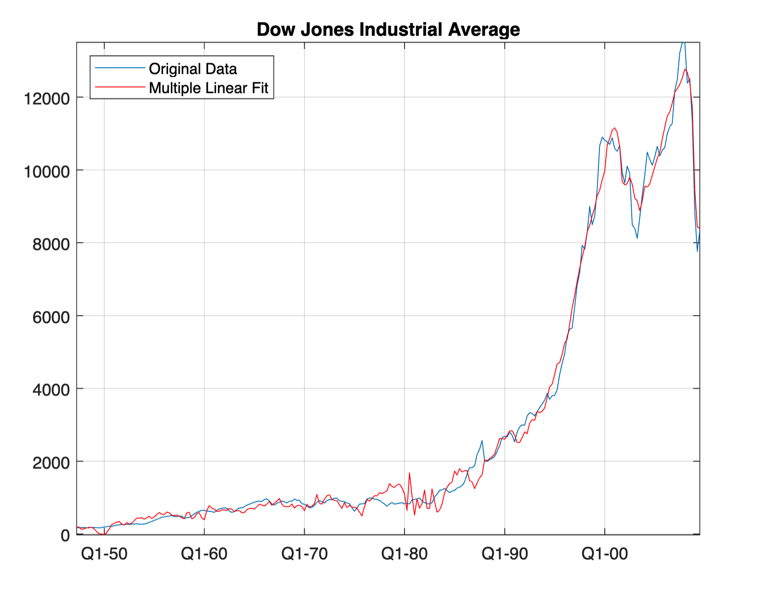
Next, we perform a fit based regression on multiple economic factor data to predict DJI movement
%% import the data
djData = readtable('djiEconModel.csv');

%% create a model to fit the data
model = fitlm(djData{:, 3:end}, djData.DJI);

%% plot the original data with the fitted values in red
plot(djData.Dates,djData.DJI)
hold on
plot(djData.Dates,model.Fitted, 'r', 'DatetimeTickFormat', 'QQQ-yy')
hold off
grid on
axis tight
title('Dow Jones Industrial Average')
legend('Original Data', 'Multiple Linear Fit', 'Location', 'NW')

%% create Rsquared containing the ordinary R-squared value
Rsquared = model.Rsquared.Ordinary;
disp(['The Ordinary R-squared value is: ', num2str(Rsquared)])
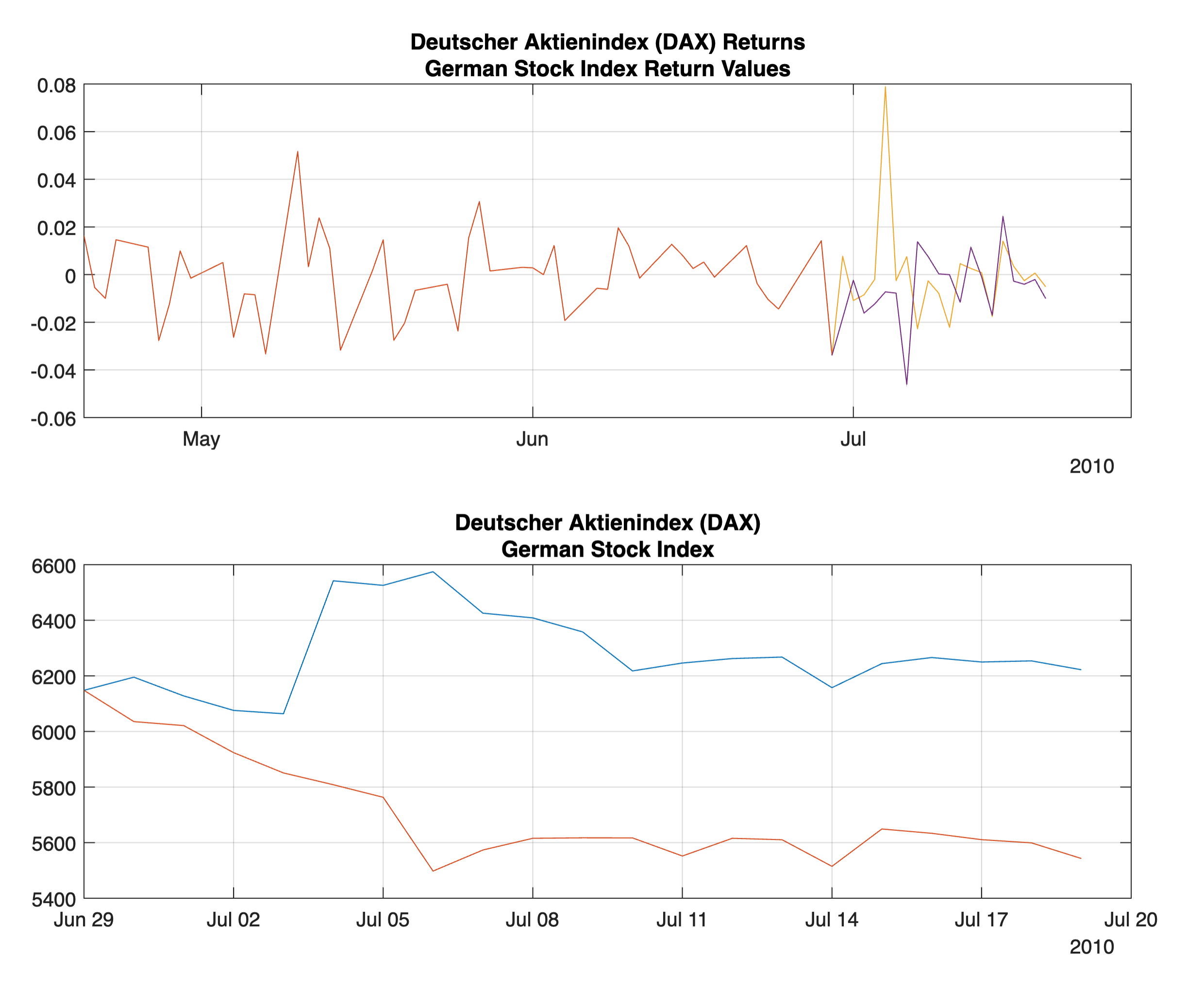
Another Monte-Carlo simulation example is using the numbers from DAX and a t Location-Scale distribution to calculate a matrix of random numbers with nSteps rows, indicating the number of days, and nExperiments columns, indicating the number of trials, named simReturns.
%% import table of returns
returns = readtable('germanStocks.csv');

%% plot original data
subplot(2,1,1)
plot(returns.Dates(end-50:end), returns.DAX(end-50:end))
hold on
grid on
title({'Deutscher Aktienindex (DAX) Returns';'German Stock Index Return Values'})

%% set-up dimensions for Monte-Carlo Simulations
nSteps = 20;            % Number of steps into the future
nExperiments = 2;       % Number of different experiments to run

%% generate random numbers from the information in DAX
tFit = fitdist(returns.DAX, 'tLocationScale');
simReturns = random(tFit, nSteps, nExperiments);

%% plot the returns
futureDates = returns.Dates(end) + days(1:nSteps);
plot([returns.Dates(end) futureDates],
     [returns.DAX(end)*ones(1, nExperiments) ; simReturns])
hold off

%% plot the Index Values
lastDAX = 6147.97;
predictions = ret2tick(simReturns, 'StartPrice', lastDAX);
subplot(2, 1, 2)
plot([returns.Dates(end) futureDates], predictions)
grid on
title({'Deutscher Aktienindex (DAX)'; 'German Stock Index'})
Miscellaneous#
Differentiate common usage of Numpy vs. MATLAB.
MATLAB basic functions can be referenced through an official cheatsheet.